Quality measures

Metrics such as elevation difference or angular difference rely on a reference DEM. This dependence can be problematic for several reasons:

Not all reference DEMs boast a high spatial resolution.
The reference DEM and the DEM under evaluation might represent different time frames, during which the area of interest could have experienced changes, be it from natural phenomena like landslides or human activities like construction.
The two DEMs could differ in spatial resolution, and resampling a DEM can introduce errors and biases, especially concerning slopes and reliefs.

Thus, introducing some methods to assess the quality of a DEM without comparing it to a reference DEM can be beneficial. Such methods are called quality measures. Two of these methods have been implemented into demcompare: the curvature and the slope orientation histogram.

Curvature

Given these potential discrepancies, it’s important to incorporate standalone quality metrics like Curvature when evaluating a DEM.

Curvature represents the second derivative of the elevation (the slope being the first derivative). For a given DEM $u$ , curvature is calculated with the formula $div(\frac{\nabla u}{ \| \nabla u \|})$ . Negative values are associated with convex profiles, whereas positive values are associated with concave profiles.

It is a really useful measure in urban areas as it highlights the restitution quality of buildings and streets. For more natural areas, it can for instance bring some light on hydrologic networks or valleys. This is illustrated in the figure bellow.

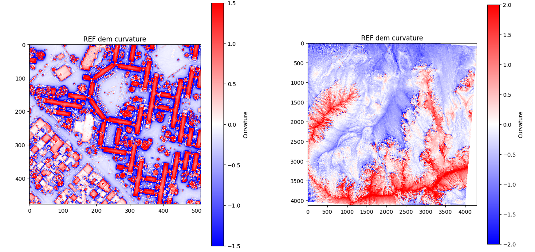
../../_images/Curvature.png — Fig. 7 Curvature for an urban DEM and a mountainous DEM. Features such as buildings, trees or valleys are easily identifiable.

Slope orientation histogram

Using the same convention with slopes as with the hillshade (0° for north orientation, 90° for east orientation…), it is possible to plot a circular distribution of the pixels according to their slope orientation. This quality measure is called the “slope orientation histogram” and it is very helpful in identifying the presence of artifacts.

For instance, it can detect if the method of DEM construction or sampling generates some slope orientations in the main direction of the interpolation grid. Therefore, it can spot the artefacts dependent on the DEM generation method, independently from the input data. An example is illustrated below with 2 DEMs, one of them containing artifacts and the other being more realistic and homogeneous.

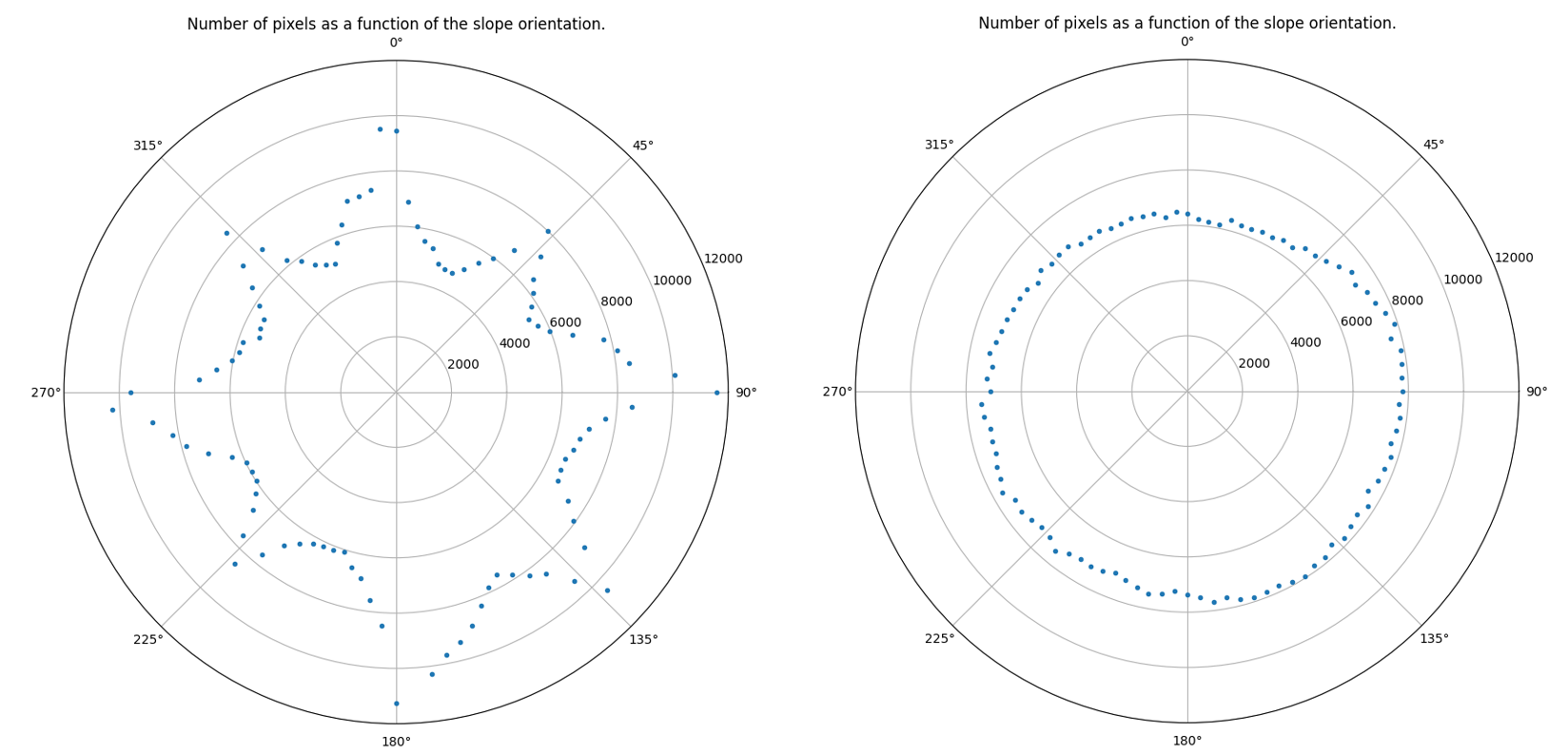
../../_images/slopeOrientationHist.png — Fig. 8 Slope orientation histogram for 2 DEMs covering the same hilly area. On the left, some artifacts can be identified in the main and secondary directions of the grid (0°, 90°, 180°, 270°, and 45°, 135°, 225°, 315°). On the right, a dominant direction of the hills can be identified toward the south-east.